TE probes benchmark from in-flight measurement

Following to 2022 first measurements & findings using XC vario, I have bought two TE probes from ESA systems last winter, to be flown & recorded over 2023 season.

• Venturi is the TE probes I have flown over years, it was my reference
  
• TE-RU is the "standart" bent TE antenna. It can be installed on tail either pointing up or down
• TE-DN is the double-head type of TE antenna. It can be installed either vertically either horizontally
  

It means the same glider can be flown in 5 differents TE Antenna configurations, for comparison purpose.

It is a bit difficult to judge from reading the instrument in flight what are the specificities for each arrangement. Still what could be nevertheless be seen is that pneumatic vario reading looked less jumpy in maneuver with either TE-RU or TE-DN in comparison to the reference TE-Venturi.

Let's see what we can learn from XC-vario recording.

As a standart maneuver, for each of the flights with a new antenna configuration I did perform a phugoid, which allows to cover a large range of airspeed in straight flight with minimum piloting input & with acceleration & deceleration.

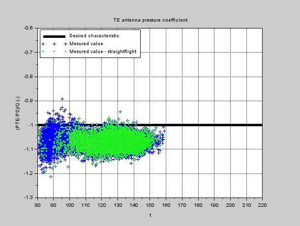
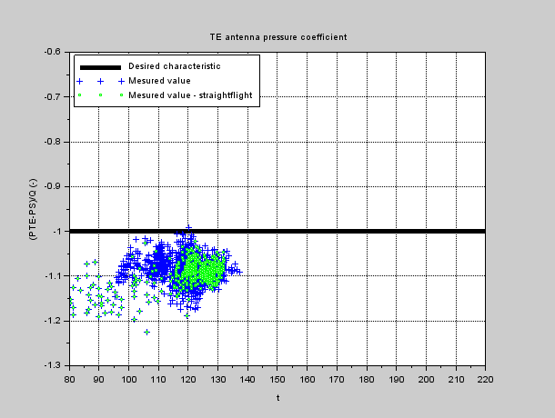
Measured pressures during phugoid

From those pressure recordings it is possible to evaluate "Antenna pressure coefficient", by combining Static pressure PS & total pressure Q along with TE pressure through :

CP_TE=(PTE-PS)/Q.

• To perfectly compensate speed variations in vario reading, from a theoretical point of view antenna pressure coefficient value should be equal to -1 .
• If pressure coefficient is above -1, antenna is undercompensating
• If pressure coefficient is below -1, antenna is overcompensating
  

(NB : the value of -0.95 is sometime stated as desired pressure coefficient value, based on pilot feedback from experiment)

Here are the results from measurements :

Antenna coefficient for the 5 configurations, in phugoid

Since anemometric system for LS6 glider is carying only small speed errors (see link) - at least for symetric flight - PS & Q can be trusted & antenna coefficient can be considered in absolute.

The following trends can be observed:

• TE-Venturi is overcompensating, by about ~7% whatever speed (as from last year analysis)
• TE-RU gives a more exact compensation when pointing down, particularly for cruise flight speeds
  
• TE-RU tends to overcompensate at lower speeds when pointing up, and undercompensate when pointing down
• TE-DN gives a more exact compensation in cruise when set horizontally, while giving a more exact compensation in low speed range when set vertically.
• TE-DN tend to undercompensate at low speed when set horizontally, and over compensate in cruise speed when set vertically

Based on straight flight analysis, both TE-RU pointing down & TE-DN set horizontally seems to be two equivalent best choices for good compensation in cruise flight.

 

Recording pressure signals over the full flights overs the opportunity for wider analysis. I have for example extracted the time history for the first thermal for flights with each configuration.

Here is the result from measurements :

Antenna coefficient for the 5 configurations, in circling

The following trends can be observed:

• The whole range of pressure coefficients seems shifted in circling compared to straight flight : it could be caused either by antenna behavior, either by error in anemometric circuit for circling conditions - since PS is used as reference for evaluating pressure coefficient.
  Second cause is likely the main driver, so it makes sense to only consider circling measurement for comparing antennas & not in absolute.
  
• For both TE-RU & TE-DN, there is less compensation difference between antenna orientations in circling phases compared to straight flight.
• TE-DN is compensating less than TE-RU in circling flight

Based on circling analysis, antenna orientation seems less critical in circling than in straight flight, but it is difficult to state for sure which antenna configuration is better compensating, due to likely static circuit errors.

All in all, I think it is clear I will not fly anymore my TE-Venturi antenna : general feeling in flight & recordings analysis goes in same direction.
Further study on the noise over pressure measurement could help choosing between TE-RU & TE-DN antennas, but will require first to sort what comes from air bumpiness from the day versus antenna behavior in the observed signal. To be continued !

On yaw string behavior

 Yaw string is a basic "equipement" of our gliders, that often questions the people out of gliding movement. My answer to such inquiry is to say "this is a low cost sideslip sensor" - with a tongue in cheek...

Well yes yawstring relates to sideslip, but at the end do we really know how much the angle we observe  every flight relates to sideslip ?

Yaw string under control...

First let's define sideslip : it is as a convention the angle between the speed vector projected into wing plane & fuselage axis - a complicated way to describe that it quantify how much sideways the glider is flying. Sideslip is most of the time called "beta" - here is a sketch.

Sideslip definition

 

Now that sideslip is defined, how much yawstring angle relates to sideslip ? 

To answer this question,  Computationnal Fluid Dynamic results (CFD) provides a good view on fuselage local aerodynamic behavior.
Below is the flow picture obtained from CFD for a typical glider at beta=+4deg of sideslip (wind blowing on the right cheek of the pilot...). 

Friction line for a typical glider with 4deg of sideslip & 4deg of aoa

 Glider skin is colored according to local pressure, and friction lines are plotted, which are showing the flow direction right onto the skin. Those lines are illustrating how much locally the airflow is being "deformed" by fuselage presence, and in particular the way it is flowing laterally in symetry plane when sideslip is present. 

We can consider that the friction line at one location on the glider is giving the orientation of yaw string placed there - given a whool string is very thin compared to glider size & very close to fuselage skin. With appropriate post processing, the angle of friction lines versus glider symetry plane can be numerically evaluated from CFD output, and used for further analysis

CFD results in several condition  have been considered, to characterize yaw string response to glider parameters. Here is the plot of for yaw string angle computed for a typical canopy location, with Aoa ranging between 0 & 8 deg, and Sideslip between 0 & 8deg as well

Yaw string angle in relation to sideslip

The following observation can be made

• Yaw string angle mostly respond to glider sideslip, and there is more yaw string angle than actual sisdeslip: yaw string is an amplifier for glider sideslip
• In term of magnitude, typical "yaw string gain" is 2.5, that is when sideslip is 1deg, yaw string angle reads 2.5deg.
  
• To a lesser extend, response of yaw string to sideslip evolves slightly with aoa - that is "yaw string gain" evolves slightly between cruise & circling phases
  

Another type of investigation can be made from CFD : when fixing the glider conditions, the gain of yaw string can be computed for various position over the glider. The following curve can be plotted, that gives the yawstring gain versus its relative positionning versus nose, in proportion to maximum height.
(e.g : Nose distance/max fuse height=0.85 on a 80cm high fuselage means yawstring is placed 0.85*90=76.5cm away from the nose)

Yaw string gain in relation to yaw string positionning vs fuselage nose

From this curve, it can be observed that the more forward on fuselage is (Nose distance/max fuse height toward 0), the greater the yaw string gain is, that is the more the yaw string amplifies the sideslip. This may help you tune the position of your yaw string, depending how much you want it to be active.

A small statistical study for yaw string positioning over 8 modern single seaters of various class, and 3 double seaters has been performed, with following findings :

• On single seater or in forward seat of double seater, yaw string generaly lies between 0.85 & 1.05 times the max fuselage height from nose, meaning yaw string gain is in the range of 2.4 to 2.6
• For the instructor seat of double seater, yawstring lies much further back, close to 2 times the max height from the nose : in that region yaw string gain is expected to be much closer to 1. That is instructor reads less sideslip from yaw string than his pupil does !

For sure there are exception to this rule when glider fuselage shape is out of the ordynary - typically yawstring gain on a Libelle would likely show a somewhat different behavior.

May be you will now look differently to your yaw string when you are flying !

TE probe characteristics

As XC Vario is recording the different pressures available on my glider, namely static PS, dynamic pressure Q & TE probe PTE, it is possible to study them.
Anemometric calibration curve of LS6 being quite good, as showing low error of IAS vs CAS, it means in particular than static measuremnt is of good quality.

DLR-measured anemo calibration curves for LS6 (1986)

As a result, it is possible to build TE pressure coefficient with a reasonable confidence in the absolute level. TE pressure coefficient is defined as follows :

CP_TE=(PTE-PS)/Q

To have a good compensation antenna, value for this pressure coefficient should be CP_TE=-1.
Now, let's see what we measure in flight on the LS6, which is fitted with a venturi-type compensation antenna. 

First, a phugoid manoeuver is showing a good range of speed with minimum stick input. Below is plotted the antenna pressure coefficient as function of indicated airspeed.

TE pressure coefficient in phugoid

It can be observed that my antenna is not a perfect, as being 5 to 10% off vs desired value for typical cruise speeds.
As pressure coefficient is more negative than desired, it means this antenna has a trend to over-compensate altitude variation for speed variations. In a typical pull up on a modern glider, speed variation  vs geometric altitude variation corresponds to a ~10m/s correction term, meaning a 5% error on the coefficient makes ~0.5m/s error on variometer reading.
As well to ne noted : when reaching low speed range, the antenna over-compensation behavior is increasing.

In real life, TE pressure is exposed to many perturbations : turbulence, sideslip, angle of attack, pilot input, etc... Ideally the local pressure coefficient would stay imune to those parameter, but this is actually  not the case. As a result, TE pressure is affected by some measurement noise, that is at the end polluting variometer readings.
Below is the TE pressure coefficient recorded over 30min during one of my XC-country flight, showing an example of "real life" situation.

TE pressure coefficient while flying in southern alps, from Col de Vars to Crete de Peyrolle

In contrast to the relatively ideal phugoid manoeuver, it can be observed that pressure coefficient versus speed is quite noisy, especially for low speed, with either over- or under-compensation behavior.
When on top we isolate points corresponding to wings levels (in green), it appears that the low speed noise is very much related to circling phase. In thermals, probability for turbulence or for non symetric flight is higher, both likely to expose TE probe to undue perturbations. Noise is less in straight flight, but does exist as well.

Below is a collection of time slices analysed from a TE antenna characteristic, to start getting a sense of statistics & patterns. From left to right & top to bottom : clound street flying, low altitude hang flying, High mountaign area flying, low start over hill in weak lift, small wave flying, landing

 Performing similar measurement for different antenna would be interesting, but was not done so far.

As a final note, it can be either concluded I have a bad TE antenna, or that reliable variometer without an antenna would be a benefit...

2022 Landing survey

 In August this year, I had a bit of a rough landing, or at least it felt as such. It was the classical LS6 trap : too slow on final approach with Landing flap configuration extended, resulting into nose up attitude in flare to compensate for quasi-stalled status, and tails hitting the ground first.

During 2022 season, quite a lot of data was recorded using the XC vario installed on the LS6. I have taken here the opportunity to have a survey on glider parameters during some of the landings, with the objective to analyse the specific rough landing event.

In a first plot, indicated airspeed is plotted over the last 30 second before touch down, as well as the difference between airspeed & ground speed (hence vertical wind profile) in the last 60m above touch down. Touch down is then hapenning @ t=0/Zp=0.

Indicated speed vs time & vertical profile of headwind

Those plots cover landings on 3 airfields : Aire sur adours in may, Moissac in July & August, St Auban end of August/beg September.  The rough landing happened on the 15th of august at my home airfield of Moissac, corresponding to red curve.

Here are some basic observations :

•  In the landings recorded, indicated airspeed reading in approach (left curves), 20sec before touch down, varies from 95kph to 120kph.
  Recordings are converging at touch down toward a 80-to-90kph narrower band.
  
• 15th of august landing (red) happened for the approach at the lowest speed
  --> 95 kph 20sec before touch down, 90kph 2sec before touch down, 80kph at touch down
  AND it resulted in a landing perceived as rough
• July flight (black) was performed with a speed almost as low
  --> 95 kph 20sec before touch down, 90kph 2sec before touch down, 85kph at touch down
  BUT it did not result in a landing perceived as rough
  
• Difference between red & black is the wind (right curves) : in july there was virtually no wind, whereas 15th of august landing happened in a moderate wind (~15kph in altitude), showing a 5 to 10kph wind gradient over the last 5m over ground

What is being taught to pupils ("you shall increased your approach speed on windy days") is here shown measurable, since very similar speed scheduling resulted in a different outcome at touchdown on a calm & on a windy day.
On the other hand, approach realised with greater speed margin repeatably led to "normal landing" feeling, even in wind up to 30kph.

More measurements are available from XC vario sensors : in a second plot, altitude & velocity time histories are presented over the last 30seconds before touch down, as well as vertical velocity, vertical accelerometer reading, pitch attitude & pitch rate in the last 5 seconds before touche down.

Time history for altitude, indicated airspeed, vertical speed & acceleration, pitch & pitch rate

Here are a few observations :

•  It looks like I tend to realise lower approach at my home airfield (red, black, green) than on other airfields...
• Like for airspeed, altitude time histories converges into a narrow band over the last 20m/10sec before touch down
• Rolling phases correspond to high noise on many sensor of XCs vario (static & differential pressures, accelerations, roations rates), corresponding both to higher excitation (runways are not always regular) and local vibration behavior for the canopy mounted XC vario instrument.
  

More specificaly related to the sensation for a rough landing :

• Red corresponds to the highest vertical speed at touch down, and black the closest to zero : it confirms the different perception at touch down for those two "low indicated speed approaches".
  
• On green curve, 3-to-2 sec before touch down there is a anticipated flare, with temporary nose up attitude resulting in vertical speed reduction.
  It constrasts with red, for which nose up attitude just before touch down seems to have had no impact on vertical speed variation rate. Likely, quasi-stalled wing status due to lower speed/higher aoa in the last seconds prevented wing lift to develop further following to pitch action, preventing fine tuning of the vertical trajectory.
  
• Accelerometer is quite shaky once the glider is rolling, easily showing +2.7G reading whatever the landing : high values of positive Az does not correspond by itself to the feeling for a rough landing.
  On the other hand, red curve shows at touch down a significantly negative reading (-2.7Gs) followed by a significant positive value (+3.1Gs). This signature is likely to results in the perception of a rough landing.
• This specific signature can be understood as follows :
  
• Red curves shows the highest pitch attitude at touch down
• A significant nose down pitch rate after touch down ishould be the signature for a tail strike.
  Negative pitch acceleration results in a negative vertical acceleration measured on the instrument panel location - but also in pilot stomach to a certain extend...
• Shortly after tail, main wheel is touching the ground as well, stopping the pitch down motion & restoring positive acceleration felt in the canopy of the glider & in pilot's stomach...

All in all, recording XC-vario parameters proved very usefull to understand what happened, recalling the basics that I was taught as a pupil in term of speed scheduling in approach...

 

Wind measurement - Observing earth boundary layer while landing

 With XCVario, several speeds are measured :

• True AirSpeed (TAS) can be reconstructed from dynamic pressure & temperature measurements.
• GPS measurement (from FLARM at this stage) gives direct access to Ground Speed (GS)

 --> Difference between both TAS & GS is then an estimate of instantaneous wind in direction of flight.

As an illustration for this, the difference between TAS & GS is plotted during final landing phase, representing earth boundary layer above the airfield.

A few observations can be made

• On the 8th of may :
  
• Both landings show a reclined boundary layer profile, with weaker wind at landing altitude than @ 20m above ground
• On the 2nd landing, wind is stronger & deeper present on the ground
  
• Gust content is rather low for both landings
  
• On the 13th of september in St Auban :
• Wind is present almost down to landing altitude, with little reduction of wind component before the last 5m of altitude
  
• @t~10-12sec, a sensible gust can be observed ~70m above landing altitude, with a "gap" of TAS not visible on GS, and roll activity.
• Another gust is visible @t~30sec, 10m above ground
• A further gust is visible during ground roll -that has been filtered out of wind speed vertical profile
  

----------------------

Landing on the 8th of may 2021 against "vent d'Autan" with no lift

----------------------

 

Landing again on the 8th of may 2021 against "vent d'Autan" after a flight in weak distorded lift

----------------------

 

 

Landing on the 13th of september 2021 in St Auban

 

Observing temperature profile while flying thermals

Temperature as well as static pressure are measured by XC vario. As a results, it is possible to plot temperature as function of pressure altitude. 

Below are plotted a few time slices as recorded. Several observation can be made :

• Flying straight in sink or neutral zone results in measuring a certain gradient of temperature versus altitude - generally steeper than -6.5deg standart atmosphere gradient.
  
• Circling & climbing in a thermal shows a similar temperature gradient versus altitude compared to measured in straight flight, but with an offset corresponding to warmer air
  
• While entering or exiting the thermal, a transition happens in the same order of magnitude : we end up drawing an hysteresis
• The greater the climb, the greater the "warm offset"
• Those observations seem to remain true for strong climb in mountain area as well as weak thermal over flat land on a poor day

Using temperature sensor as a "thermal sniffer" is not the objective here, nevertheless collecting this data could be worthwhile  in term of validating weather models - particularly if coming from a network of gliders flying the same area.

 ----------------------

 Strong thermal at Malaup montain on the 13th of september 2021

• Transition
  
• 3.95m/s mean value over 850m climb
• Transition
  

 

 ----------------------

Good thermal at La Molière (north Vercors) on the 13th of september 2021

• Transition in a uplift area, then sink
  
• 2.1m/s mean value over 320m climb
• Transition
  

 

 

 ----------------------

Soft climb at Gache mountain on the 13th of september 2021

• Transition
  
• 1.1m/s mean value over 370m climb
• Transition
  

 ----------------------

Weak thermal over flat land on the 9th of october 2021

• Transition
• 0.6m/s mean value over 100m climb
• Transition 

Recording with XC Vario

 As described in the former post, XCVario has onboard sensors of interest to analyse flight paths of a glider. With two other pilots, Jean-Luc & Guy-François, we are working on formulas & algorithms using those sensors to provide enhanced variometry measurement.

As a first step, Jean-Luc & Guy-François have created a fork from XCVario software, that is providing in particular the emission on Bluetooth for parameters of interest, that can be recorded by a smartphone. Over the season, I could record more than a ten of flight hour on my LS6 glider, that can be analysed on over the winter. A typical 5hrs flight results into ~30Mo of text file. For analysis purpose I use Scilab cripts (open source cousin for Matlab...), but Guy François has also developped his own post processing program.

Looking into this recorded material is providing interesting insight into the condition encountered while flying. Further post will be dedicated to observing what is measured

A Cross country flight over the alps (see the flight in Weglide)